COVID19 R0 tracker

Summary
Date	03/2020-?
Tags	COVID19, python
Partners	Houda K. https://twitter.com/sha3kouka
Contribute?	https://discord.gg/TPsPJCJ
Learn more	Original work by lisphilar: https://www.kaggle.com/lisphilar/covid-19-data-with-sir-model

The work around this project is still ongoing. Lisphilar contacted me after finding this webpage, he invited us to join him and contribute. We are currently working on the connections between the various measures (lockdown, masks, social distancing, etc…) taken at different times in different countries to mitigate the spread of the virus and the values of the SIR/SIRF-F/SEWIR parameters during the pandemic. The project now involves data analysis (maybe even some Machine Learning?), Natural Language Processing to analyze a massive dataset will the measures of all countries since the beginning of the pandemic, and a bunch of other interesting things. Interested ? Join us here.

The goal of this project is to evaluate the now infamous \(R_0\) (and \(R_e(t)\)) for various countries daily, and more specifically for Canada, Québec and Morocco. I’ve been interested in knowing the \(R_0\) value for various places but was surprised by how hard it was to do so. After some research, Houda K. and myself found the excellent ipython notebook by lipshar that provides all the tools necessary to (1) perform minimizations over various SIR models to get their current parameters and (2) plot one of those SIR models given some parameters (this second point is often confused with a prediction).

SIR-F: R0 evolution by country

	Last_update
0	10/16/2020 21:23

R0 worldwide view

R0 Evolution

Alberta Algeria Angola Argentina Australia Austria Belgium Brazil British Columbia Cameroon Canada Chad Chile China Cuba Djibouti Ecuador Egypt Finland France Germany Guatemala Iceland India Iran Italy Ivory Coast Japan Jordan Kenya Mauritania Mexico Morocco Niger Nigeria Ontario Pakistan Panama Peru Philippines Quebec Russia Saskatchewan Senegal Slovenia Somalia South Africa South Korea Sweden Taiwan Thailand Tunisia Turkey US Ukraine Venezuela Zimbabwe

If you are looking for the most recent minimization of the whole SIR-F parameters, use this link to directly jump there.

Theory

SIR: Susceptible Infected Recovered

The SIR model is a simple mathematical model that relies on differential equations to model the evolution of each group - Susceptible to the virus/disease, Infected by the virus/disease and Recovered/Removed (this category includes both individuals who recover and those who die from the disease) - which actually means modelling the spread of the virus.

The model thus divides an initial population \(N\) (fixed) of individuals into three different groups that will vary through time:

• \(S(t)\): those Susceptible but not yet infected by the virus
• \(I(t)\): those who are currently Infected (and infectious)
• \(R(t)\): those who have Recovered from the virus/disease and now have immunity to it (they cannot get infected again and are not infectious anymore)

The model is supposed to describe the change in the population of each of these groupes using two parameters, \(\beta\) and \(\gamma\). \(\beta\) describes the effective contact rate, which impacts the rate of individuals that move from group \(S\) to \(I\), while \(\gamma\) describes the mean recovery rate which impacts the rate of inidividuals that move from \(I\) to \(R\). Our model can thus be represented this way:

\[\mathrm{S} \overset{\beta I}{\longrightarrow} \mathrm{I} \overset{\gamma}{\longrightarrow} \mathrm{R}\]

The system of differential equations that describe this model were first provided by Kermack and McKendrick in 1927 (see sidebar Resources):

\[\begin{align} \frac{\mathrm{d}S}{\mathrm{d}t} &= - \frac{\beta \cdot S(t)}{N} \cdot I(t) \\ \frac{\mathrm{d}I}{\mathrm{d}t} &= \frac{\beta \cdot S(t)}{N} \cdot T(t) - \gamma \cdot I(t) \\ \frac{\mathrm{d}R}{\mathrm{d}t} &= \gamma \cdot I(t) \\ N &= S(t) + I(t) + R(t) \end{align}\]

The unit effective contact rate \(\beta\) is \([\frac{1}{\text{unit of time}}]\). An infected individual comes into contact with \(\beta\) other individuals per unit time (of which the fraction that are susceptible to contracting the disease is \(\frac{S}{N}\)).

The unit mean recovery rate \(\delta\) is also \([\frac{1}{\text{unit of time}}]\). An infected individual will remain infectious for a mean period of \(\frac{1}{\gamma}\).

We now have our SIR model. But where’s the \(R_0\) ?

SIR: R0

This is where things can become confusing… When you read \(R_0\) somewhere for the COVID19, it’s usually very hard to determine which \(R_0\) is meant in that case. \(R_0\) is defined as the basic reproduction number and can be computed as:

\[R_0 = \frac{\beta}{\gamma} = \frac{\text{effective contact rate}}{\text{mean recovery rate}}\]

\(R_0\) is the number of seconday infections that one infected person would produce in a fully susceptible population through the entire duration of the infectious period.

\(R_0\) is important becase it conveniently provides a threshold condition for the stability of the disease-free solution:

• If \(R_0 < 1\) : the solution to the problem will be a stable asymptote, meaning that the disease will definitely di out
• If \(R_0 > 1\) : the solution to the problem will be unstable and diverge, meaning that an outbreak occurs

\(R_0\) is supposed to be fix over time as it is supposed to be evaluated after an epidemic outbreak. However, \(R_0\) is also affected by the behavior of a population during an outbreak, it is thus possible to estimate a local \(R_0\) at different moments of an outbreak by considering a significant portion of the data (weeks or months) to estimate the SIR parameters over that period of time.

Re(t)

Another important parameter of an epidemic outbreak is \(Re(t)\) which is the effective reproductive number.

\(Re(t)\) represents the number of secondary infections that one infected person would produce throught he entire duration of the infectious period

Notice that the difference with \(R_0\) is that \(R_0\) considers a fully susceptible population, thus:

\[Re(t) = R_0 \cdot \frac{S(t)}{N}\]

\(Re(t)\) describes wether the infectious population increases of not:

• If \(Re < 1\) : the infectious population is receeding
• If \(Re > 1\) : the infectious population is increasing

A common issue is that sometimes, people consider the amount of persons who died because of the virus/disease in the Recovered group thus, the \(R_0\) obtained is different. A model such as the SIR model can be used to model rates of individuals transiting from various groups to other, the definition of each group is often problematic and blurry (for example what does “Recovery” mean? each country has a different definition). Another problem is that the SIR model is only one of several epidemic models, and their \(R_0\) definitions are different (see later).

Example of SIR model

We can now choose a set of parameters for our model and plot it, to better understand what it looks like. We’ll mode a disease with a \(R_0=2.0\) that propagates in a population of 1.78 million individual (like the city of Montreal).

\[\begin{align} N &= 1 780 000 \\ \beta &= 0.2 \\ \frac{1}{\gamma} &= 10 \\ R_0 &= 2.0 \end{align}\]

Which we can then plot :

Such an outbreak would take 150 days before reaching a peak of 250 000 infected. It would take more than 200 days to clear the outbreak out of the city that would infect about 1.5 million individuals out of the initial 1.78 million. Notice that there are no mentions of individuals who die because of the virus for this model.

SIR-D: SIR + Deaths

It is possible to extend the SIR model by considering the number of people that die because of the disease. If we do so, our new model looks like:

\[\begin{align*} \mathrm{S} \overset{\beta I}{\longrightarrow}\ & \mathrm{I} \overset{\gamma}{\longrightarrow} \mathrm{R} \\ & \mathrm{I} \overset{\alpha}{\longrightarrow} \mathrm{D} \\ \end{align*}\]

We are now considering two possible outcomes for infected individuals: Recovery or Death.

We thus have a new parameter, \(\alpha~ [ \frac{1}{\text{unit of time}}]\) that represents the mortality rate of Infected individuals.

We are not however going to be spending too much time on this model, we’ll directly move on to the next one, SIR-F, which is the one we’ll be using.

SIR-F: Fatal and unconfirmed

Due to the high rate of mortality in the case of COVID19, it is reported that Susceptible individuals sometimes die without being confirmed as Infected. However, we can assume that Deaths because of COVID19 will eventually be reported.

To consider this possibility, we will first start by considering a new group in our population \(S^*\), a group of individuals who are infected without being reported as such. These individuals can die without passing by the Infected group. We can thus consider this possibility by extending our model this way:

\[\begin{align*} \mathrm{S} \overset{\beta I}{\longrightarrow} \mathrm{S}^\ast \overset{\alpha_1}{\longrightarrow}\ & \mathrm{F} \\ \mathrm{S}^\ast \overset{1 - \alpha_1}{\longrightarrow}\ & \mathrm{I} \overset{\gamma}{\longrightarrow} \mathrm{R} \\ & \mathrm{I} \overset{\alpha_2}{\longrightarrow} \mathrm{F} \\ \end{align*}\]

Which is described by the following system of equations:

\[\begin{align*} & \frac{\mathrm{d}S}{\mathrm{d}t}= - \frac{\beta \cdot S(t)}{N} \cdot I(t) \\ & \frac{\mathrm{d}I}{\mathrm{d}t}= (1 - \alpha_1) \cdot \frac{\beta \cdot S(t)}{N} \cdot I(t) - (\gamma + \alpha_2) \cdot I(t) \\ & \frac{\mathrm{d}R}{\mathrm{d}t}= \gamma \cdot I(t) \\ & \frac{\mathrm{d}F}{\mathrm{d}t}= \alpha_1 \cdot \frac{\beta \cdot S(t)}{N} \cdot I(t) + \alpha_2 \cdot I(t) \\ & N= S(t) + I(t) + R(t) + F(t) \\ \end{align*}\]

The previous parameter \(\alpha\) will now have to be changed into two disting parameters, one to describe the mortality rate of the Infected cases, and a second one for the deaths without being confirmed.

\(\alpha_1~[-]\) that is uniteless represents the mortality rate of the undected cases from the \(S^*(t)\) population

\(\alpha_2~[ \frac{1}{\text{unit of time}}]\) that represents the mortality rate of Infected individuals

SIR-F: R0

In this case, the basic reproduction number \(R_0\) can be defined using its definition:

\[R_0 = (\text{contacts per unit time}) \cdot (\text{proba of transmission per contact}) \cdot (\text{duration of infection})\]

Which can be written in the case of the SIR-F model as:

\[R_0 = \beta \cdot (1 - \alpha_1) \cdot (\gamma + \alpha_2)^{-1}\]

SIR-F: Example

We can thus plot the model (I actually did not plot this one, the plot is from the lipshar notebook - see sidebar resources) for a \(R_0 = 2.5\), an initial population of \(N = 1 000 000\) and a some arbitrary parameters:

Note that the model this time considers the individual that die because of the virus (wether confirmed or not). Since the number of Deaths is reported and consequent in the case of COVID19, considering this additional feature for our model will help better fit the model for each country.

SIR-F model fit

Methodology

Now that we understand how the SIR, and more specifically SIR-F, models work; we can try to use them to evaluate the current value of \(R_0^{SIR-F}\) and \(R_e^{SIR-F}(t)\). Actually, since the outbreak is ongoing, we cannot really measure \(R_0^{SIR-F}\) as it is suposed to be the value for the whole outbreak. In our case, what we can do is measure \(R_0^{SIR-F}(t)\) to estimate the relative evolution of the outbreak for each country.

Let’s clarify our methodology through an example.

The data

The raw data used in this proect mostly comes from the John Hopkins University CSSE COVID19 Github repository (except for the data for Québec, which is sourced from Wikipedia). The data available in this repository is not perfect (it is actually “broken” for several countries, data is missing for several others, …) but it is an ongoing work that benefits from the updates of thousands of people. The repository provides the daily Confirmed cases, Deaths and Recoveries for various countries, provinces, cities and places (some cruise ships for example).

If we pull the data for Canada for example (as of the 4th of May), it looks like this:

We have our Confirmed cases, Deaths and Recoveries.

Relevant time interval

We previously mentionned that the model parameter values, such as \(R_0^{SIR-F}\) will change during the epidemic as people’s behavior will change (more hand washing, social distancing, confinment/lockdown measures, …). Thus, the current parameters of the disease might be very different from the parameters at the beginning of the disease. We are interested in evaluating the current parameters of the disease. If we were to use the complete data we have for Canada since the very beginning of the outbreak, we will not get the parameters for the current parameters as they will be affected by the behavior we had at the beginnig of the outbreak (that changed since then). Thus, the first thing we will do is to try to guess when is the last time that the model parameters changed significantly.

We are here going to assume that a change in the parameters of the models/disease can be reflected by a signfiicant change in the rate of infections.

We will thus use a tool designed to detect significant trend changes in a dataset. The following figure presents the result of such an algorithm (the quality of the plot is not great as it is not used, the data regarding the last trend changepoint is directly extracted using python, it is shown here to help the reader understand the process).

In the case of our plot for Canada, it is possible to see that the algorithm assumed that the latest significant trend change happened the 20th of April. We will thus try to minimize the values of our SIR-F model over the available data between the 20th of April and today, the 4th of May.

Another solution would have been to run the minimization over a moving window of 7 days since the very beginning of the outbreak and to compute the \(R_0\) value for each 7 days window. However, since the minimization process takes more than an hour for 25 countries on an i5 laptop, the current solution was prefered.

SIR-F minimization

We can now perform our minimization over the time interval we determined. The minimization results are presented in the following table:

	score	alpha1 [-]	1/alpha2 [day]	1/beta [day]	1/gamma [day]	country	start_date	end_date	susceptibles	total_population	R0(t)	Re(t)
SIR-F	0.0	0.1	1132.0	11.0	17.0	Canada	20Apr2020	04May2020	34349218.0	37855939.0	1.3	1.2

Let’s try to interpret the parameters:

• score: score is the residual of the minimization process, always good to keep an eye on your residual just in case it did not converge this time. As you can see, it did converge this time.
• \(\alpha_1~[-]\): Mortality rate of the undetected cases. In other words, portion of undetected infected that die, the other portion \((1-\alpha_1)\) will survive this first stage and become part of the Infected group. The model believes that this parameter’s value is \(0.1 (~=~10~\%)\)
• \(\frac{1}{\alpha_2}~[ \text{day} ]\): Mortality rate of Infected individuals. The model assumes that 1132 infected individuals die per day.
• \(\frac{1}{\beta}~[ \text{day} ]\): The effective contact rate. The model currently assume that each infected person comes in contact with \(\frac{1}{\beta} = 11\) other individuals per day.
• \(\frac{1}{\gamma}~[ \text{day} ]\): The mean recovery rate. The model currently assumes that it takes \(\frac{1}{\gamma}=17\) days for an Infected individual to Recover (which is quite close to some of the values estimated by Chinese doctors at the beginning of the outbreak)
• \(R_0(t)\): Currently at \(1.3\), we’re almost there but not yet
• \(R_e(t)\): Currently at \(1.2\), we’re almost there but not yet (a little bit more)

Since the situation is changing everyday, it is necessay to run the minimization process everyday and to re-evaluate the parameters. For this reason, I will update this page on a regular basis. It would also be interesting to visualize the current prediction of the model and to evaluate the evolution of \(R_0\) over several weeks. Lucky you, I’ve been running this script for more than 20 countries every day since the 19th of March (the process will keep computing new values every day as they come).

SIR-F: R0 evolution

We can thus take a look at the evolution of \(R_0\) with a short term representation of the model’s prediction (remember to be careful with these predictions as they assume constant values for the model parameters in the future, which we know is not true).

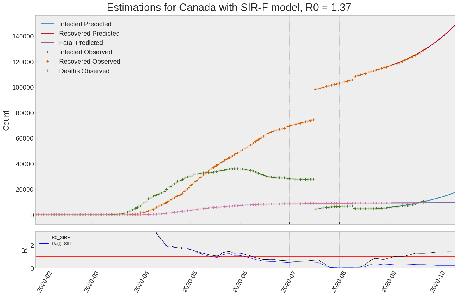
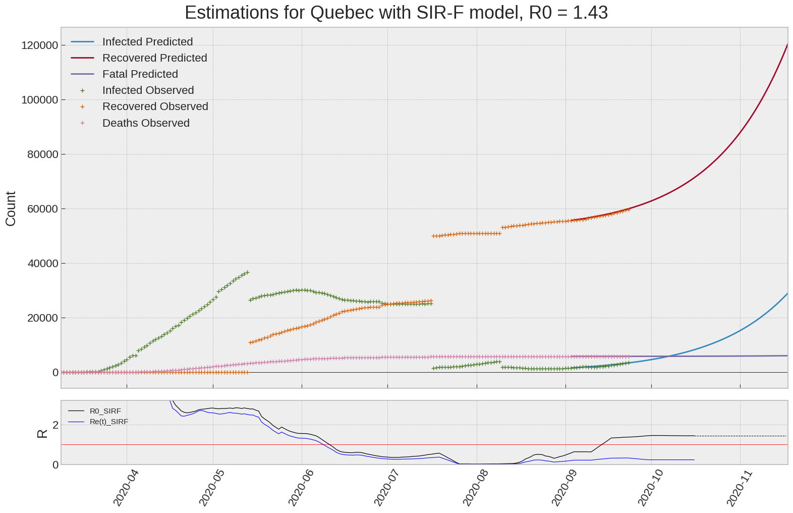
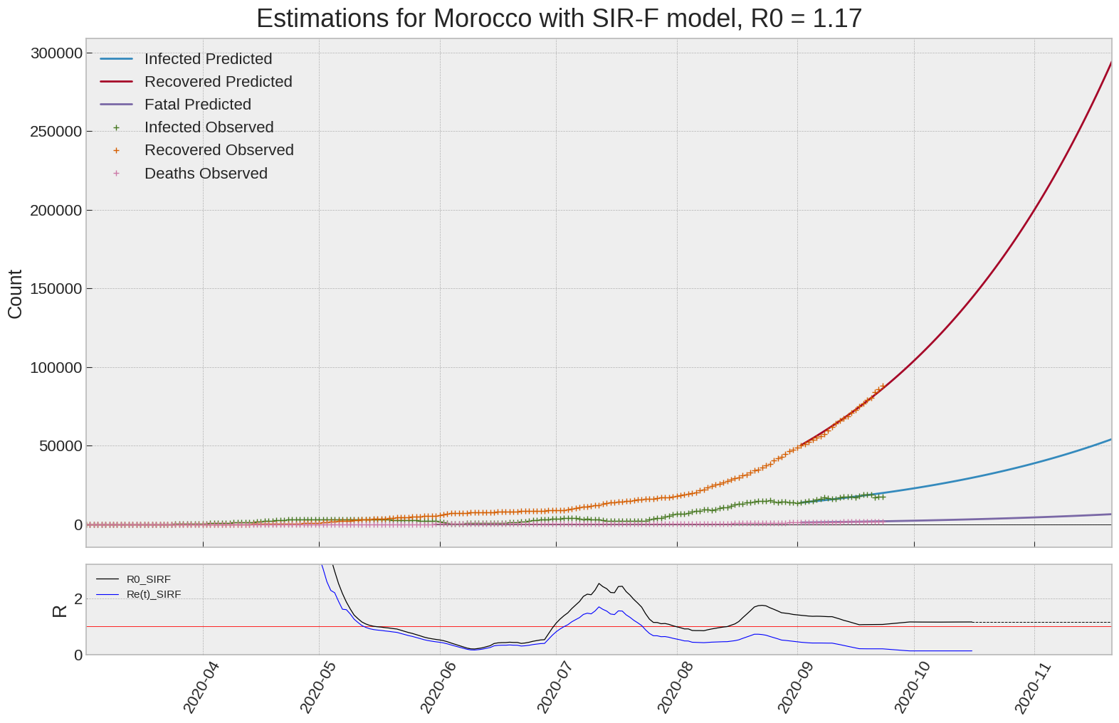
It is possible to see on the plot above the raw data in addition to the SIR-F model prediction using the parameters we previously presented. Under this chart, it is possible to see the evolution of \(R_0\) (this tiny plot is the most interesting IMO as it shows the progress done).

Finally, the last thing we can do is to plot the whole model with the curent parameters for a longer term period (over months/years):

If we do so for Canada, it is possible to see that the model currently assumes that there will be a second wave (as \(R_e(t)\) is still not smaller than \(1\) this was to be expected) that should start around the end of Summer, beginning of Fall.

Remember: all of this is just modelling, it can be useful at best, it is not a prediction of the future. It can definitely help guide our decisions and evaluate the progress accomplished. These models CANNOT be used to “predict” how the outbreak is going to play out. We need to check the data everyday.

R0 evolution for Canada, Québec and Morocco presented with a 20 days forecast.

SIR-F parameters minimization

Forgot the meaning of the parameters ?

	Last_update
0	10/16/2020 21:23

SIR-F scores

country	R0	Re(t)	alpha1 [-]	1/alpha2 [day]	1/beta [day]	1/gamma [day]
Somalia	0.0	0.0	0.8	1548	15182	141
Djibouti	0.0	0.0	1.0	0	17	22
Cameroon	0.0	0.0	0.7	58	9426	0
Egypt	0.2	0.1	0.1	1667	79	14
Niger	0.2	-0.1	0.7	21	27	0
Australia	0.3	-0.1	0.2	1638	53	19
South Korea	0.5	0.2	0.0	4565	27	13
Nigeria	0.5	0.4	0.0	3156	77	40
Senegal	0.5	-0.5	0.0	5878	76	39
Kenya	0.6	0.2	0.0	3188	121	70
Ivory Coast	0.7	-0.2	0.0	38232	11	8
Japan	0.7	0.6	0.0	7381	16	12
Mauritania	0.8	-4.6	0.0	3650	16	12
Iceland	0.8	-65.5	0.0	8627	17	13
South Africa	0.8	0.4	0.0	1877	30	25
Pakistan	0.8	0.7	0.0	1972	13	11
Peru	0.8	0.0	0.0	8241	21	18
Guatemala	0.8	-0.7	0.0	911	14	12
China	0.9	0.8	0.2	5671	16	17
Panama	0.9	-5.9	0.0	21542	35	31
Mexico	0.9	0.7	0.1	1756	7	7
Brazil	0.9	0.8	0.0	735	14	13
Cuba	1.0	-1.7	0.0	1066	11	11
Chile	1.0	-0.7	0.0	1254	8	8
Alberta	1.0	0.2	0.0	1951	10	10
Russia	1.1	0.8	0.0	1749	28	31
Argentina	1.1	0.3	0.0	2066	10	12
Venezuela	1.1	0.0	0.0	1118	9	11
India	1.1	1.1	0.0	817	10	11
Morocco	1.2	0.1	0.0	3990	8	9
Germany	1.2	0.7	0.0	5885	13	16
Iran	1.2	0.7	0.1	8686	13	17
Algeria	1.4	0.3	0.0	1477	46	66
Canada	1.4	0.2	0.0	6023	9	13
Turkey	1.4	0.8	0.0	5383	13	20
Quebec	1.4	0.2	0.0	9629	7	10
Thailand	1.5	0.8	0.0	1117	35	54
Ontario	1.7	0.3	0.0	11115	8	14
Austria	1.8	-4.7	0.0	8760	9	16
US	1.9	1.7	0.0	6762	97	188
British Columbia	1.9	0.3	0.0	731	19	39
Zimbabwe	2.0	-1.9	0.0	2247	48	104
Jordan	2.0	-4.7	0.0	1341	7	15
Slovenia	2.1	-30.0	0.0	2506	10	21
Chad	2.1	-2.4	0.0	521	7	17
Ukraine	2.6	0.6	0.0	1510	27	74
Italy	2.6	1.3	0.0	26286	23	62
Taiwan	2.7	-0.9	0.2	37745	15	50
Saskatchewan	2.8	0.4	0.0	5663	8	22
Philippines	2.9	2.0	0.0	1197	22	70
Angola	4.4	-0.3	0.0	2483	26	126
Finland	7.4	-35.3	0.1	161	19	0
Tunisia	10.9	-19.2	0.0	3042	15	178
Ecuador	19.1	-17.4	0.4	463	14	0
France	23.1	11.7	0.0	8179	31	787
Belgium	35.4	-63.3	0.0	28746	67	2605
Sweden	36.1	-77.2	0.0	18974	501	0